I-EEG User Guide
This guide covers project setup, signal review, preprocessing, computations, annotations, and result export.
1. Getting Started
1.1 Create a Project
Choose File > New Project..., then:
- Select an EEG/iEEG recording.
- Choose a location for the
.ieegproject file. - Click Confirm.
Supported formats: .edf, .bdf, .fif, .vhdr, .set, and .cnt.
The project links to the original recording; it does not copy the raw data.
1.2 Open a Project
Choose File > Open Project... and select an .ieeg file. The application restores the project state described in Section 8.1.
2. Main Window
2.1 Overview
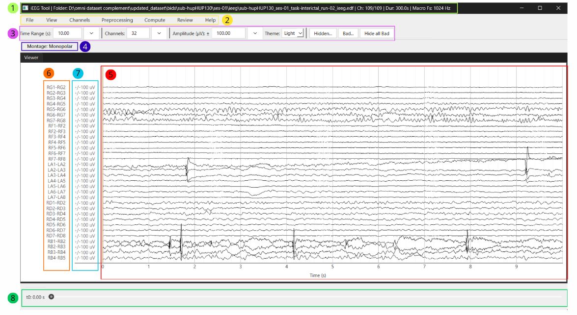
- Window title and recording summary: path, channel count, duration, and sampling rate
- Menu bar
- Display toolbar
- Active montage/reference
- EEG/iEEG signal viewer
- Channel labels
- Amplitude axis in µV
- Time-navigation bar
Trace colors identify channel state: Micro channels are blue and confirmed bad channels are red. Red takes priority when a Micro channel is also bad.
2.2 Menu Bar
- File: create, open, save, or close a project; exit the application
- View: zoom, reset the view, or use Scalogram mode
- Channels: assign Macro or Micro groups
- Preprocessing: select a montage/reference, configure display filters, or open the PSD
- Compute: run REI, Gamma Spike, or HFO analysis
- Review: add annotations
- Help: open this guide or the shortcut list
2.3 Display Toolbar
- Time Range (s): seconds shown
- Channels: traces shown at once
- Amplitude (µV): visual scale; it does not change data or results
- Theme: Light or Dark interface
- Hidden...: restore hidden channels
- Bad...: review or clear bad-channel marks
- Hide all Bad: hide every bad channel
- Edit Bipolar...: edit the montage; visible only in Bipolar mode
Enter a value or use the available choices for time range, channel count, and amplitude.
3. Explore the Recording
3.1 Navigation
3.1.1 Channels
Scroll over the viewer or use:
- Up/Down Arrow: move through channels
- Shift + Up/Down Arrow: move faster
- Ctrl + Up/Down Arrow: move much faster
3.1.2 Time
Drag the bar below the viewer or use:
- Left/Right Arrow: move through time
- Shift + Left/Right Arrow: move faster
- Ctrl + Left/Right Arrow: move much faster
3.2 View Menu
3.2.1 Zoom Selection
Choose View > Zoom Selection, then drag a rectangle over the required time and channels. Press Escape before releasing to cancel.
Double-click the viewer to return one zoom step. Choose View > Reset Zoom to restore the view that preceded the zoom sequence.
3.2.2 Scalogram Mode
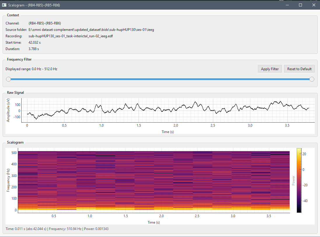
Choose View > Scalogram Mode, then drag horizontally across one channel. The new window shows the channel context, raw signal, time-frequency map, frequency filter slider, and hover values. Very short selections are ignored.
Press Escape before releasing to cancel.
4. Manage Channels
4.1 Macro and Micro Groups
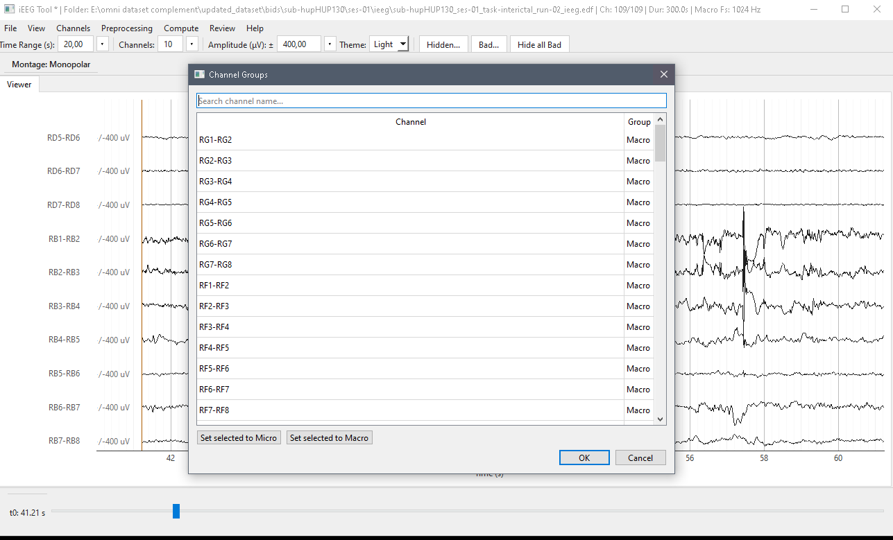
All channels are Macro by default. Choose Channels > Channel Groups..., select rows, click Set selected to Micro or Set selected to Macro, then click OK.
Groups control channel styling, filter profiles, and the Macro/Micro PSD panels. In the main viewer, Micro channel traces and labels are blue; Macro channels use the default theme colors.
4.2 Select Channels
Click a trace or label to select it. For multiple channels:
- Ctrl + click: add or remove one channel
- Shift + click: select a range
- Ctrl + Shift + click: add a range
4.3 Hidden Channels
Right-click selected traces and choose Hide. Use Hidden... to restore them. Hiding affects visibility only; it does not delete data.
4.4 Bad Channels
Right-click selected traces and choose Mark as bad. If all are already bad, choose Unmark as bad. Use Bad... to review marks or clear them all.
Bad status is application-wide: changes in the viewer or PSD appear in both. A bad trace is red and remains visible until hidden; red takes priority over the blue Micro-channel color. Bad displayed channels are excluded from computation lists.
Hidden and bad are separate states: restoring a hidden bad channel does not clear its bad mark, and unmarking a channel as bad does not make a hidden channel visible.
5. Preprocessing
5.1 Montage / Reference
Choose Preprocessing > Montage / Reference, then select:
- Monopolar: display each imported channel
- Bipolar: display automatic
Channel 1 - Channel 2derivations - Average: subtract the shared channel average
- Median: subtract the shared channel median
- Common Reference...: subtract one selected physical channel
Average and Median exclude bad channels from the reference pool. Samples covered by a Bad segment annotation are masked during reference calculation. Hidden channels remain in the pool.
Automatic Bipolar Montage
Bipolar mode extracts each label's electrode prefix and contact number, groups contacts by electrode, sorts them numerically, and pairs consecutive contacts. For example, A1, A2, and A3 produce A1-A2 and A2-A3. Each displayed trace is the actual signal Channel 1 minus Channel 2.
Unrecognized labels and non-consecutive contacts are skipped. The application reports skipped contacts, warns if no pair is possible, and asks for confirmation if imported labels already look bipolar.
Bad-Channel Behavior
Automatic generation uses the raw bad-channel state present when Bipolar mode is selected. A pair is omitted if either source contact is bad. If A2 is bad, neither A1-A2 nor A2-A3 is created; the software does not bridge the gap with A1-A3.
While Bipolar mode is active, marking A1-A2 as bad marks the derived trace only. The pair remains visible in red and is excluded from computation lists; raw A1 and A2 are not immediately marked. Use Hide or Hide all Bad to remove the trace from view. Hiding does not change the montage or bad-channel state.
When leaving Bipolar for Monopolar, Average, Median, or Common Reference, each bad derived pair is converted to its first source contact: bad A1-A2 becomes bad A1; A2 is not marked. Existing raw bad contacts remain bad. Returning to Bipolar then excludes every automatic pair containing A1.
Changing bad status does not rebuild the montage currently on screen. After unmarking a raw contact, regenerate pairs by switching away from Bipolar and selecting it again, or choose Edit Bipolar... > Back to default > OK. Hiding a raw contact does not exclude it from automatic pairing.
Edit Bipolar Montage
The Edit Bipolar... button is available only in Bipolar mode. Use it to change Channel 2, add pairs, restore automatic pairs, apply with OK, or discard with Cancel.
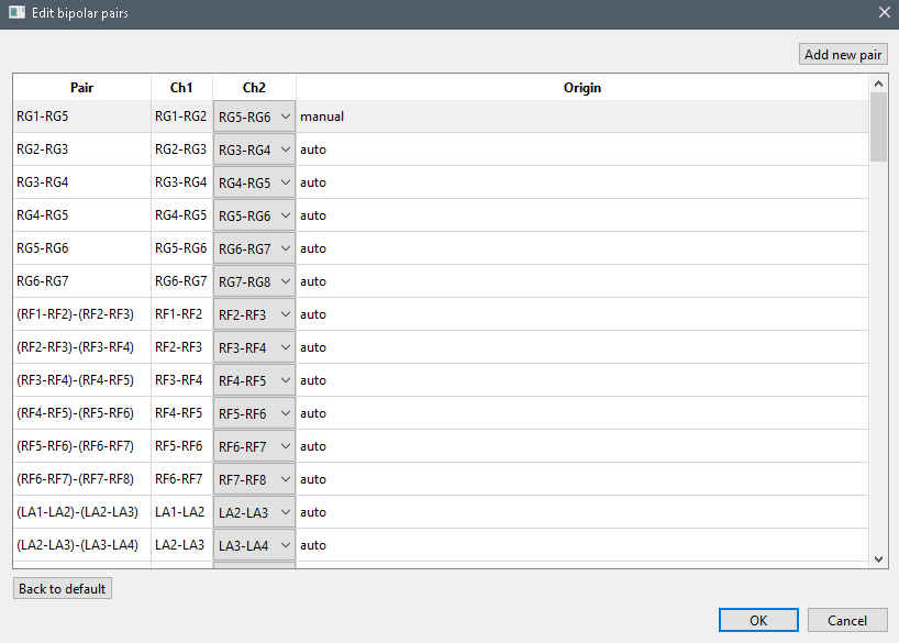
Raw contacts marked bad are excluded from the available Channel 1 and Channel 2 choices and from the automatic montage restored by Back to default. Unmark a raw contact before opening the editor if it must be used in a pair.
Validation and Warnings
Channel 1 and Channel 2 must differ, and bipolar names must be unique. Invalid edits are not applied.
A pair spanning two recognized electrode groups triggers a Cross-electrode bipolar pairs warning. Choose Cancel or Keep edit.
Cancel leaves the current montage unchanged. Keep edit allows an intentional cross-electrode pair; the warning is not an error.
5.2 Display Filters
Choose Preprocessing > Display Filters... to show or hide filter controls above the viewer.

Use Scope to edit:
- All: Macro and Micro profiles
- Macro: Macro channels only
- Micro: Micro channels only
Each profile has numeric High Pass (Hz) and Low Pass (Hz) controls and Notch choices: Off, 50 Hz + harmonics, or 60 Hz + harmonics. Enter 0 to disable a cutoff; numeric fields cannot be empty.
Click Apply filters to apply the profile or Back to default to clear it. Active cutoffs must be below Nyquist, and high pass must be lower than low pass.
Filters are non-destructive. The montage/reference is applied first, then the relevant Macro or Micro profile. A padded interval is filtered before the requested window is displayed to reduce edge artifacts.
The PSD uses these profiles. Computations use separate bandpass rules; only algorithms that explicitly say so reuse the notch choice.
5.3 Power Spectrum
Choose Preprocessing > Power Spectrum, enter start and stop times, and confirm. Stop must follow start, and both values must be inside the recording. The PSD opens beside the main viewer.
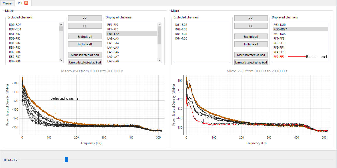
Macro and Micro Panels
The tab contains independent Macro and Micro panels based on Section 4.1. Group changes refresh an open PSD. In Bipolar mode, a pair follows Channel 1's group.
Each panel has its own channel lists, selection, plot, and zoom state. Channels use their group's display-filter profile. Power is shown in dB/Hz against Hz.
The Excluded channels list is on the left and Displayed channels on the right. If group assignments change while the tab is open, both panels update automatically. A Micro panel remains empty until at least one channel is assigned to Micro.
Curves and Channel Status
All group channels initially appear, including hidden and bad channels.
- Select displayed channels and click
<<to exclude them from that PSD plot. - Select excluded channels and click
>>to restore them. - Exclude all and Include all affect only the current panel.
- Click a name or curve to emphasize it.
- Double-click a plot to restore its default range.
PSD exclusion does not hide a trace or change its group. Bad channels appear in red. Mark selected as bad and Unmark selected as bad update the same state used by the main viewer.
Clicking a curve or displayed-channel name makes it active. Its label and curve are emphasized; a selected bad channel has a thicker red curve. Macro and Micro plots keep independent zoom states.
PyQtGraph mouse controls provide zoom and pan. They affect visualization only. The context menu is disabled, so built-in auto-range and export actions are unavailable.
6. Compute
6.1 Computation Panel
Choose Compute > Open Computation Panel, or right-click selected channels and choose Open Computation Panel. The dock can be moved, resized, or floated. It analyzes the open recording.
Shared Controls
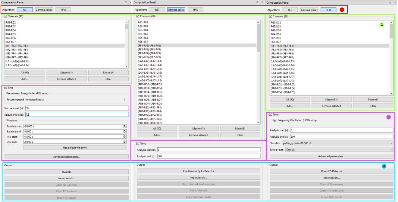
Follow the panel from top to bottom:
- Choose an algorithm: REI, Gamma Spikes, or HFO.
- Choose channels: select the signals to analyze.
- Define the analysis: enter the time interval, then review the algorithm-specific settings and Advanced parameters... when available.
- Run the algorithm: monitor progress or cancel if required. Review and export controls become available only after a successful run or import.
- Review the outputs: inspect the main-viewer overlays, channel summary, and event or heatmap views provided by that algorithm. Complete any manual event corrections before export.
- Export the results: this creates the persistent result folder. Use Import results... later to reopen that folder with the matching recording and montage.
The Time and Output areas adapt to the selected algorithm. Import is also available before a new run.
Use All, Macro, or Micro to replace the list with non-bad channels from that scope. Use Add..., Remove selected, or Clear to edit it. Verify the list after changing montage/reference. The signal is extracted using the montage/reference active when the run starts.
Confirmed bad channels are unavailable for selection. Display high-pass and low-pass filters are not reused unless an algorithm explicitly includes them in its preprocessing.
Export and Import Results
After review, use the algorithm's Export button to save tables, metadata, and a README; REI also exports its heatmap. Export again after manual corrections. File > Save does not replace result export.
To reopen results, first load the matching recording and montage, then click Import results... and select the exported folder. The algorithm is detected automatically and its summaries, reviews, and overlays are restored. Import rejects incompatible data and replaces the current result, so export unsaved reviews first.
6.2 Recruitment Energy Index (REI)
Definition, Origin, and Validation
REI estimates how early and strongly each channel is recruited at seizure onset. It combines baseline-normalized high-frequency energy with recruitment time, then assigns a score and rank. Higher scores indicate earlier, stronger recruitment relative to the analyzed channels.
REI adapts the EI implementation in BrainQuake, an Apache-2.0-licensed project, based on the scientific method of Bartolomei et al. (2008). Its current settings combine BrainQuake's 60–140 Hz band with the fourth-order filtering and 10σ threshold also used in Alfredo Lucas's IEEG_EI. BrainQuake uses fifth-order filtering and 20σ; IEEG_EI uses a 70–140 Hz band. Both upstream cores use 0.5-second energy and 0.25-second scoring windows.
Eva Ozturk's contribution is adapting and connecting this computation to the application's channel/montage selection, preprocessing, editable time windows, visualizations, review workflow, and exports. The application does not use IEEG_EI's GUI or login workflow. The recorded code provenance through IEEG_EI remains acknowledged; the absence of an explicit license for its changes is documented in the third-party notices. Attribution does not resolve that permission gap.
Local numerical safeguards and window handling also differ from the upstream code. Numerical parity and clinical validation are not documented for this GUI implementation. REI is a review aid, not a clinical conclusion.
Time
Enter Seizure onset and Seizure offset. Onset sets these defaults:
- Baseline: 70 to 10 seconds before onset
- Ictal: 5 seconds before to 20 seconds after onset
Click Use default windows to restore them. REI has no minimum seizure duration. Offset must follow onset. Both windows must be non-empty and inside the recording. Baseline must end at or before onset; ictal must start at or before onset and end no later than seizure offset. Shorten invalid default windows.
For example, if a seizure ends less than 20 seconds after onset, shorten the default ictal window so it ends no later than the entered offset. If onset occurs early in the recording, move or shorten the baseline so it remains within the available data.
Preprocessing and Advanced Parameters
REI uses the active montage. Bipolar is recommended. With another montage, choose Switch to Bipolar, Run Anyway, or Cancel. Switching stops the launch so you can verify the channel list. REI uses the active signal representation and does not add a common-average reference.
REI ignores display high/low-pass values and applies a zero-phase, fourth-order Butterworth bandpass, default 60–140 Hz. Analysis band can be edited by the user in Advanced parameters....
Changes apply to the next run; there is no separate Save button. The lower value must be positive and below the upper value, and the upper value must be below Nyquist. Threshold sigma (10), energy window (0.5 s), and HFER window (0.25 s) are shown for reference but are fixed.
REI reuses each channel's Macro/Micro notch choice. If notch is off for all selected channels, the application warns about possible line-noise effects.
Confirmed bad channels are excluded. With mixed Macro and Micro selections, each channel uses the notch profile assigned to its own group.
Computation
REI is calculated independently for each selected, non-bad channel:
- Estimate high-frequency energy. The filtered signal is squared and smoothed with a fixed 0.5-second window in both the baseline and ictal intervals.
- Normalize to baseline. Each channel's baseline and ictal energy time series are divided by that channel's mean baseline energy. The resulting series is the normalized high-frequency energy ratio (HFER).
- Set a channel-specific threshold. For channel
i:
Tᵢ = max(Eᵢ,baseline) + 10 × σᵢ,baseline
Eᵢ,baseline is the normalized baseline HFER series and σᵢ,baseline is its standard deviation.
- Find recruitment onset. Recruitment is the first ictal-window sample whose HFER is strictly greater than
Tᵢ. If a channel never crosses its threshold, its onset is assigned to the end of the ictal window. Recruitment delay is reported relative to the entered seizure onset, so it can be negative when the ictal window begins before seizure onset. - Measure recruitment magnitude. For every channel, mean HFER is measured over a window of up to 0.25 seconds beginning at the earliest recruitment detected across the analyzed channels. The window is shortened if it reaches the ictal-window end.
- Combine magnitude and timing. Channels are ordered by recruitment onset and assigned an inverse timing rank
1/rᵢ, where rank 1 is the earliest. The raw score is:
REIᵢ,raw = √(HFERᵢ × 1/rᵢ)
- Normalize the scores. Raw scores are divided by the largest raw score in the current run, producing REI values from 0 to 1. The channel with the highest final REI receives final Rank 1.
The timing rank used inside the formula and the final REI rank are different: the first reflects recruitment order; the second orders the combined normalized scores. Scores are relative to the channels and windows in the current run and should not be compared as absolute values across separate seizures.
NaN or infinite raw scores are replaced with zero. If every score is zero, the result remains all-zero and should be treated as non-informative; the GUI does not automatically exclude the recording.
Run and Results
Click Run REI. Status and elapsed time update in the background. Cancel REI run requests cancellation; the current filtering step may finish first. Cancellation preserves the last completed result.
Main Viewer
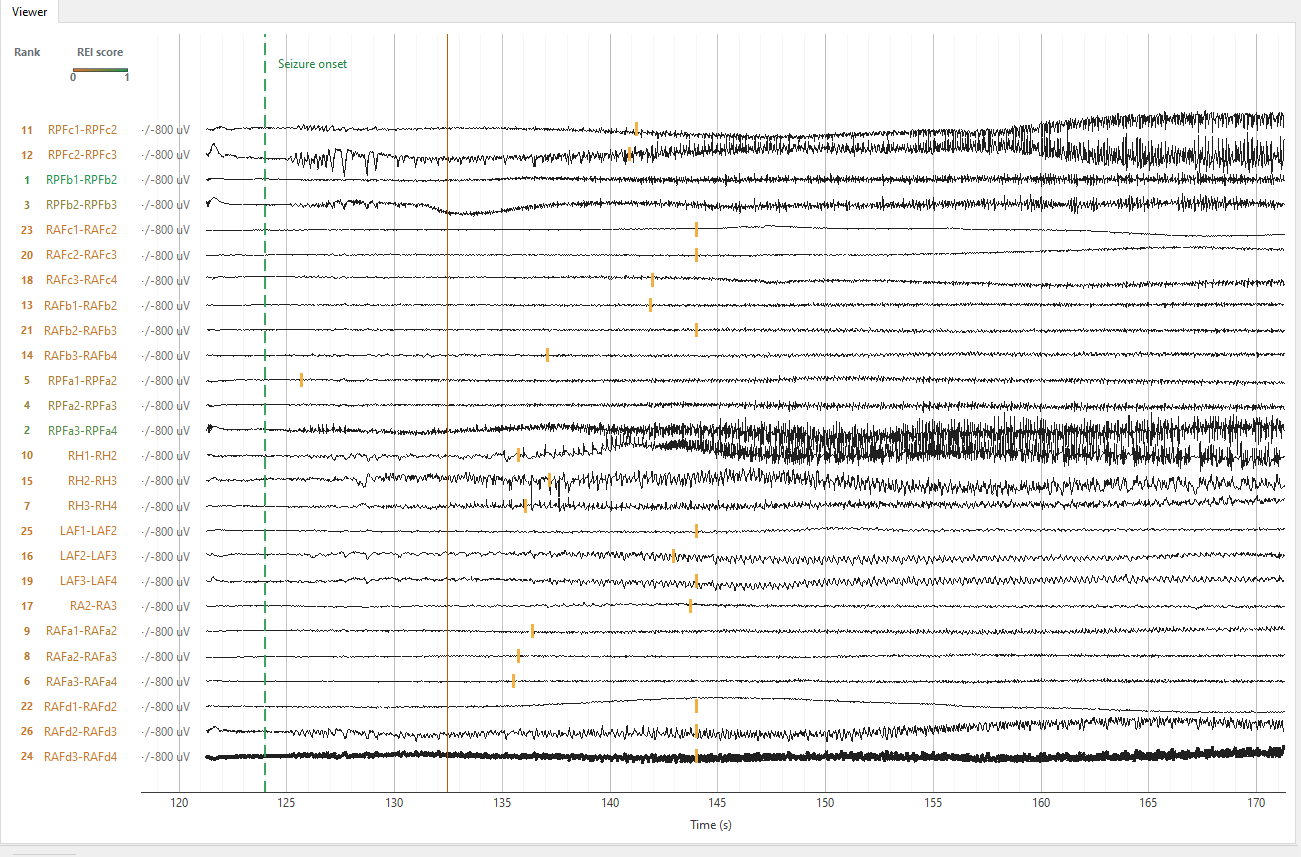
The viewer adds each analyzed channel's rank and colors its label from orange (lower score) to green (higher score). An orange tick marks visible recruitment time. Excluded channels receive no overlay.
The marker is placed at the estimated recruitment time, not at the entered seizure onset. It appears only when that time lies inside the visible window.
Channel-Level Summary
Open REI summary shows one sortable row per channel. Selecting a row selects and centers that channel in the main viewer.
Click a column header to sort the summary. The analyzed channels in the main viewer immediately follow the same order; channels not included in the REI run remain after them. Clicking a numeric header again reverses the order. The Channel header alternates between the current display order and alphabetical order. Sorting changes presentation only; it does not recalculate REI values.
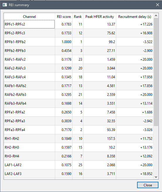
- Channel: analyzed channel or bipolar derivation
- REI score: normalized score from 0 to 1 within this analysis
- Rank: descending score order; rank 1 is highest
- Peak HFER activity: maximum baseline-normalized ictal high-frequency energy
- Recruitment delay (s): time relative to seizure onset; negative is before onset
Scores and ranks are normalized within the current channel set. Changing channels, time windows, montage, or frequency limits can change them; compare separate runs cautiously.
Heatmap
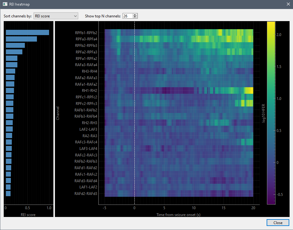
Open REI heatmap shows log10 HFER over the ictal window and a score bar plot. Sort by score, delay, peak/mean HFER, original order, or name. Show top N channels limits rows. These controls affect visualization only.
Heatmap time is expressed relative to seizure onset. Sorting or limiting rows does not change scores or exported values.
Export
Export REI results creates:
rei_summary.csv: one row per channel with its group, normalized REI score, final rank, recruitment time relative to seizure onset, and peak HFERrei_heatmap.csv: numeric HFER values by channel, with time-column headers in seconds from the start of the ictal windowrei_heatmap.png: log10 HFER heatmap with time relative to seizure onsetrei_metadata.json: source, montage, seizure timing, baseline/ictal windows, sampling rate, channel counts, filters, and parametersREADME.txt: file, value, and unit definitions
6.3 Gamma Spikes
Definition, Origin, and Validation
Gamma Spike analysis detects interictal spikes, measures associated 30–100 Hz activity, and classifies events as gamma or non-gamma.
Eva Ozturk translated the Gamma Spike algorithm, as implemented by John Thomas and colleagues in Lab-Frauscher/Spike-Gamma, from MATLAB into Python and integrated it into this software. The workflow uses the Janča Hilbert-envelope spike detector.
Time
Enter a non-empty interval inside the recording. The full recording is selected by default.
Preprocessing
Gamma Spike uses the active montage and ignores display high/low-pass values. It reuses each channel's Macro/Micro notch choice and warns if notch is off for all selected channels.
Detection and boundary estimation use an internal 10–60 Hz band; gamma measurement uses 30–100 Hz. Boundary and gamma signals use zero-phase, fourth-order Butterworth filters.
Gamma Spike has no advanced-parameter dialog. Its detection bands, thresholds, and segmented-processing settings follow the translated reference workflow and are not user-editable.
Run and Results
Click Run Gamma Spike Detector. The interval is processed in 10-minute chunks to limit memory use. Each chunk includes up to 10 seconds of overlapping signal before and after it. This temporary padding reduces filter-edge artifacts. Only events from the central 10-minute interval are retained, preventing duplicates when chunks are merged before boundary and gamma calculations.
Progress and estimated time are shown. Cancel gamma run stops an active run and preserves the last completed Gamma Spike result.
Main Viewer
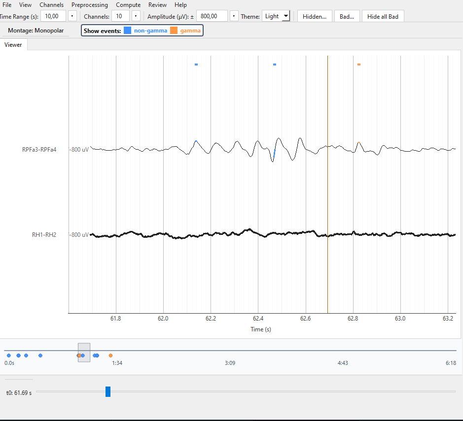
Each P1–N2 interval is highlighted on its waveform and as a bar above the viewer: blue for non-gamma and orange for gamma. Events also appear on the full-recording timeline. P1 is spike onset, N1 the main peak, and N2 spike end.
The non-gamma and gamma checkboxes change visibility only. Click a highlight or top bar to open the event in the spike grid. Click a timeline event to jump to it.
The timeline also marks the current viewer window. Hiding a class does not delete events, alter classifications, or change exported results.
Channel-Level Summary
Open channel-level summary provides sortable rows and All spikes, Gamma only, and Non-gamma only filters.
The main viewer follows the order of the rows currently shown in the summary. Sorting a column or changing the summary filter updates that order; filtered-out and non-analyzed channels remain afterward. This changes presentation only and does not reclassify events.
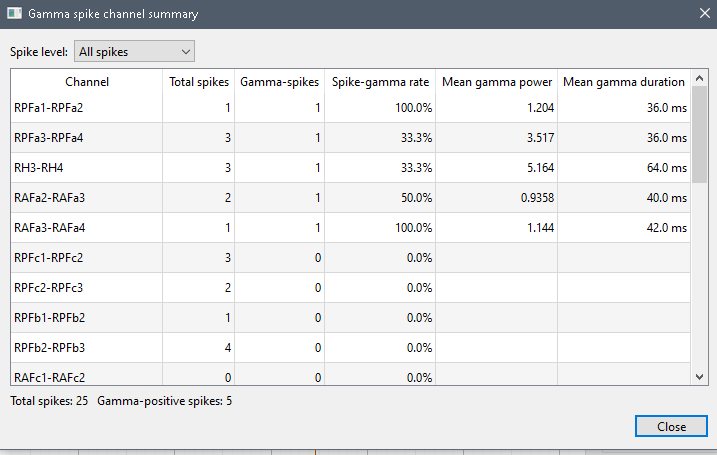
Gamma only keeps channels with at least one officially gamma-classified spike. Non-gamma only keeps channels with no officially gamma-classified spike. These controls filter rows; they do not reclassify events.
- Channel: analyzed channel or bipolar derivation
- Total spikes: retained events after post-processing
- Gamma-spikes: events whose official class is gamma
- Spike-gamma rate:
Gamma-spikes / Total spikes × 100; 0% if none - Mean gamma power: mean finite 30–100 Hz amplitude for official gamma events, in native units
- Mean gamma duration: mean selected gamma-episode duration in ms
Mean values are blank when no finite measurement exists.
Spike Grid and Manual Review
Open spike grid shows cards filterable by class, channel, and minimum gamma power.
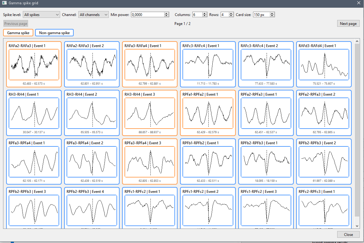
Select one to view raw and 30–100 Hz signals, time-frequency content, P1/N1/N2, gamma measurements, and the gamma window. Review plots do not alter measurements.
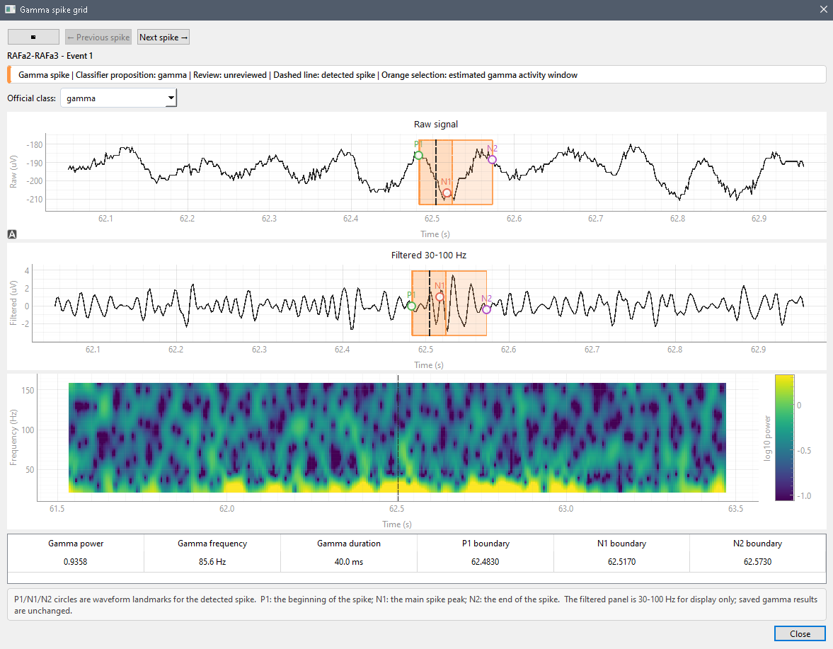
Page and layout controls support large result sets. The 30–100 Hz review trace is a visualization and is separate from the saved measurements.
Set Official class to gamma, non-gamma, or unclassified. Changes are immediate, mark the event reviewed, and update viewer overlays. There is no separate Save button or bulk classification.
The official class replaces the algorithmic class in summaries and viewer filters; the original algorithmic class remains stored for traceability. Events are reviewed one at a time.
Manual changes exist only in the current result; project saving does not preserve them. Finish review before export and export again after later changes. Closing, importing, or running a replacement result can discard unexported changes.
Export
Export gamma results creates:
gamma_channel_summary.csv: per-channel counts, rate, mean power, and mean duration using official classesgamma_spike_events.csv: channel, event number, timing, 1-based samples, algorithmic/official/manual classes, P1/N1/N2 in samples and seconds, gamma measurements, review status, and errorsgamma_metadata.json: source, analysis interval, sampling rate, chunk/context settings, notch configuration, channel/event counts, completed measurements, and timingsREADME.txt: file, unit, indexing, context, and filter definitions
Per-event heatmaps are not exported; they remain available in the spike grid.
Summary counts use the official classes present at export, including manual corrections. Export again if a class changes afterward.
6.4 High-Frequency Oscillations (HFOs)
Definition, Models, and Validation
HFO analysis detects candidate high-frequency events, classifies them, and presents them for review. Every route uses selected channels, the active montage and notch settings, one or more candidate detectors (STE, MNI, or Hilbert), shared duration/edge rules, and the same review/export interface.
The detectors, classifiers, and pretrained checkpoints are upstream work. Eva Ozturk integrated and adapted these components to the application's configuration, data handling, visualization, manual review, and export interfaces; this work does not claim new detector algorithms or model training. Component-specific terms, including academic-use restrictions and unresolved reuse permissions, are described in the third-party notices.
The candidate detector locates possible events; the selected model classifies them. Choosing the same detector across routes does not make their preprocessing or classifications equivalent.
Routes differ in preprocessing, supported band, sampling behavior, classifier, checkpoints, and classes. Results are not interchangeable. Sources: pyHFO pyBrain and Omni-iEEG.
- pyhfo_pybrain — 80–500 Hz: default when installed; native sampling; original pyHFO Model A and Model S. Lower rates work only when Nyquist supports the band; above 1000 Hz is required for the complete 80–500 Hz band.
- pyhfo_omni_legacy — 80–300 Hz: Omni legacy pyHFO route; requires at least 1000 Hz and processes at 1000 Hz.
- eHFO — 80–300 Hz: Omni artifact, spike, and eHFO three-model route with official checkpoints; requires at least 1000 Hz and processes at 1000 Hz.
pyhfo_pybrain and pyhfo_omni_legacy need Model A/Model S, not bundled with this application. Until installed, both routes are disabled in the classifier dropdown and eHFO is used by default. See README.md for what to download and where to place it.
These implementations are intended to follow their stated software routes, but that correspondence has not yet been systematically tested and does not constitute independent scientific or clinical validation. Below 1000 Hz, prefer a compatible pyhfo_pybrain band and interpret comparisons cautiously.
The 1000 Hz threshold is enforced for both Omni routes. For pyhfo_pybrain, the selected upper frequency—not the model name alone—determines Nyquist compatibility.
Time
Enter a non-empty interval inside the recording. The full recording is selected by default; all models use the same controls.
Preprocessing and Advanced Parameters
Choose a model and band. Defaults are 80–500 Hz for pyhfo_pybrain and 80–300 Hz for Omni models. Ripples 80–250 Hz and Custom (experimental) are available for all routes; Fast ripples 250–500 Hz is pyhfo_pybrain-only.
For a custom band, select Custom (experimental) and edit Low frequency and High frequency under Advanced parameters.... Click Save for the next run. Custom bands are outside the documented default configurations, may reset after restart, and appear only under All ranges in result filters.
In Advanced parameters..., enable one or more STE, MNI, or Hilbert detectors and edit their parameters. At least one must remain enabled. The application validates band limits, event duration, merge gap, minimum cycles, and detector settings.
Disabling a detector preserves its parameter values but excludes it from the next run. Detector selection changes candidate generation for every model and can therefore change both event counts and classifications.
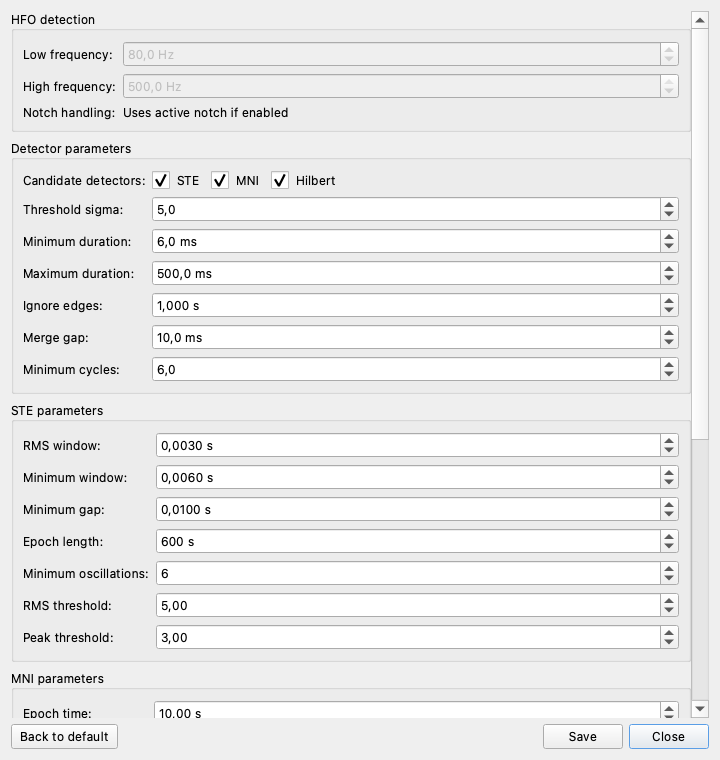
The shared controls are:
- Low / High frequency: detection-band boundaries; editable only for Custom (experimental)
- Candidate detectors: enable STE, MNI, Hilbert, or any combination
- Threshold sigma: shared fallback detection threshold, measured in standard deviations
- Minimum / Maximum duration: shortest and longest retained candidate
- Ignore edges: interval removed from both ends to avoid incomplete events
- Merge gap: maximum separation for joining nearby detections
- Minimum cycles: minimum oscillations required for a candidate
Detector-specific settings take priority over the matching shared fallback. Their concise meanings are:
- STE: RMS window controls envelope smoothing; minimum window and gap control event duration and merging; epoch length divides long data for processing; minimum oscillations sets the cycle count; RMS and peak thresholds set detector sensitivity.
- MNI: epoch time divides the analysis; epoch CHF and percent CHF define continuous high-frequency activity; minimum window and gap control duration and merging; threshold percentile sets detection sensitivity; baseline segment, shift, threshold, and minimum define baseline estimation.
- Hilbert: SD threshold sets envelope sensitivity; minimum window sets event duration; epoch length divides long data for processing.
Lower thresholds or shorter duration rules usually produce more candidates. These settings affect reproducibility and comparison with the reference workflows; keep the defaults unless changes are justified and recorded. Click Save to use changes in the next run. Back to default restores the built-in values in the dialog but still requires Save; Close discards unsaved changes.
HFO analysis uses the active montage and each channel's Macro/Micro notch choice. It excludes bad channels and ignores display high/low-pass values. Events exceeding maximum duration or lying in analysis-edge padding are excluded before classification and counted in metadata.
The padding rule prevents incomplete events at the selected interval boundaries from entering classification. Boundary exclusions are reported separately from active candidates.
Run and Results
Click Run HFO Detector. All models show progress and estimated time. Cancel HFO run requests cancellation between steps; the active detector or classifier may finish first. Cancellation preserves the last completed result.
Main Viewer
Each event is highlighted on its waveform, above the viewer, and on the full-recording timeline. Official-class colors are:
- Artifact: red
- HFO / non-spike HFO: blue
- spkHFO / spike-HFO: green
- eHFO: teal
- spk-eHFO / spike-eHFO: violet
- Unclassified: gray
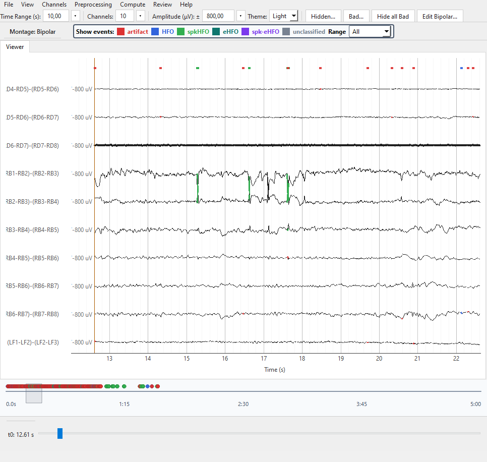
eHFO and spk-eHFO are available only for results produced by the eHFO model. They are omitted from the main-viewer legend, result filters, manual-classification choices, and channel-summary export columns for pyhfo_pybrain and pyhfo_omni_legacy results.
Deleted events are hidden. Class checkboxes and Range change visibility only. Click a highlight or top bar to open the event grid; click a timeline event to jump to it.
The timeline marks the current viewer window. Visibility filters do not change official classes, summary counts, or exports.
Channel-Level Summary
Open HFO summary shows sortable rows. Filter by All channels, At least one HFO, or At least one spkHFO. Selecting a row selects its viewer channel.
The main viewer follows the order of the rows currently shown in the summary. Sorting a column or changing the summary filter updates that order; filtered-out and non-analyzed channels remain afterward. This changes presentation only and does not reclassify events.
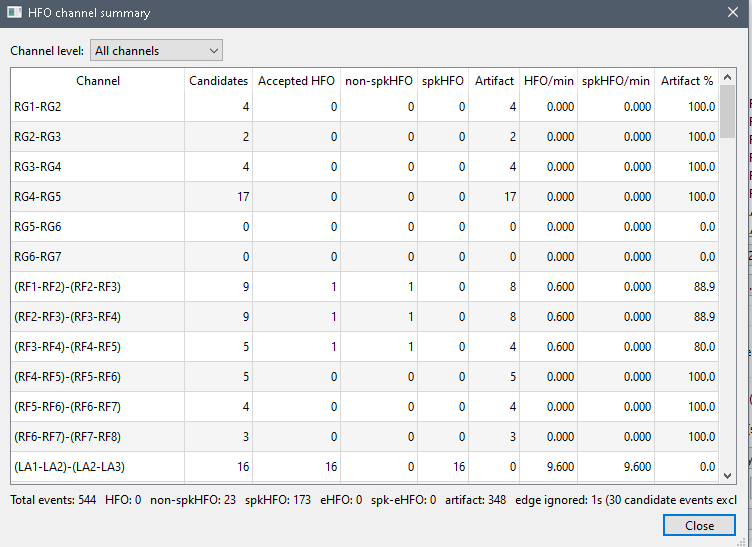
At least one HFO keeps channels with an accepted event. At least one spkHFO keeps channels with an accepted spike-associated event. Filters use official classes and exclude deleted events.
- Channel: analyzed channel or bipolar derivation
- Candidates: active candidates; deleted events excluded
- Accepted HFO: official HFO, non-spike HFO, spike-HFO, eHFO, or spike-eHFO events
- non-spkHFO: accepted events without spike association
- spkHFO: accepted events with spike association
- Artifact: official artifact events
- HFO/min and spkHFO/min: count divided by analysis duration in minutes
- Artifact %:
Artifact / Candidates × 100; 0% if none
The footer reports totals and boundary exclusions. Counts use current official classes.
Rates use the selected analysis duration, not the summed duration of detected events. Artifact percentage uses active candidates as its denominator, so deleting or reclassifying an event can update both the numerator and denominator shown in the summary.
Event Grid and Manual Review
Open HFO event grid shows cards filterable by channel, class, frequency range, and channel/time order.
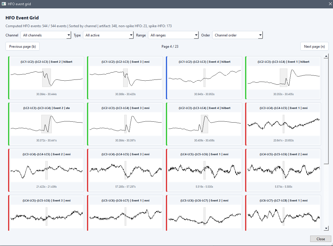
Select one to inspect signals, spectrogram or FFT, timing, band, detector, classifier proposition, available probabilities, class, and review status. Display controls do not recalculate events.
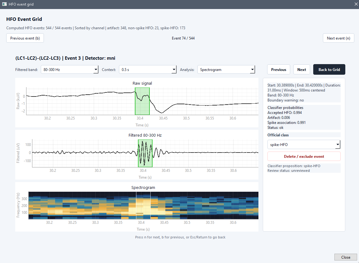
When available, probabilities include accepted-HFO, artifact, and spike association. The filtered-band, context-window, spectrogram, and FFT controls affect review visualization only and do not alter stored event boundaries or measurements.
Set Official class to artifact, HFO, non-spike HFO, spike-HFO, eHFO, spike-eHFO, unclassified, or deleted. Changes apply immediately; the original proposition remains stored. Delete / exclude event removes an event from overlays and summaries but keeps it in the exported event table.
Manual changes update the main-viewer highlight and timeline immediately. Deleted events remain exportable so the original candidate and the review decision can be audited.
There is no separate Save button. Project saving does not preserve HFO results or reviews. Finish review before export and export again after later changes.
Running another HFO analysis or importing a different HFO result replaces the current in-memory result. Export reviewed results before either action.
Export
Export HFO events creates:
hfo_channel_summary.csv: per-channel candidate, accepted, non-spike, spike-associated, eHFO, artifact, deleted, and boundary counts; rates and artifact percentagehfo_events.csv: identity, timing, sample indices, duration, detector, band, input/detection sampling rates, probabilities, propositions, official/manual classes, review status, boundary flags, and errors; deleted events remain includedhfo_metadata.json: source, interval, sampling rates, model, detectors, parameters, notch settings, montage/reference, exclusions, classifier origin/status, and review totalsREADME.txt: file, column, class, sampling, preprocessing, and unit definitions
7. Review Menu
7.1 Annotate
Choose Review > Annotate, then:
- Select the annotation type and scope.
- Add an optional note.
- Click OK.
- Drag over the required interval.
Scope can be the clicked channel, selected channels, or all channels. Press Escape before placement to cancel.
Right-click an annotation to edit or delete it. The Annotations dock lists existing annotations; select one to jump to it.
Viewer context actions apply to the annotation region under the pointer. Deleting an annotation removes it from both the viewer and the dock.
8. File Menu
8.1 Save
Choose File > Save. The .ieeg project stores:
- raw-file link; annotations; hidden/bad channels; Macro/Micro groups
- edited bipolar pairs for later Bipolar use
- Macro/Micro display filters; time range; visible-channel count; amplitude scale
- selected computation algorithm and channels
- REI seizure timing, baseline/ictal windows, and frequency limits
- Gamma Spike and HFO analysis intervals
- HFO model, band, detector selection, and advanced parameters
- latest REI result metadata, when available
It does not store:
- active reference mode; projects reopen in Monopolar
- complete REI, Gamma Spike, or HFO results
- Gamma Spike or HFO manual event reviews
- Light/Dark theme or main-viewer time position
- open docks, review grids, PSD/scalogram windows, or other secondary windows
- Gamma Spike/HFO class and range visibility filters
Restore results and viewer overlays with Import results... and a matching export folder.
Save the .ieeg project for review configuration and annotations; export each computation for complete scientific results. These operations are complementary.
8.2 Save As
Choose File > Save As... to save the same state to a new .ieeg file.
Use Save As... when the project has no path or when creating a separate project copy. It does not copy the linked raw recording.
8.3 Close Project
Choose File > Close Project to keep the application open without a project. If changes are unsaved, choose to save, discard, or cancel.
8.4 Exit
Choose File > Exit to quit. Unsaved changes trigger the same confirmation.
9. Help Menu
9.1 User Guide
Choose Help > User Guide to open this page in the default browser.
9.2 Shortcuts
Choose Help > Shortcuts to open the keyboard and mouse shortcut list.
10. Practical Review Workflow
- Create or open a project.
- Inspect the recording in Monopolar mode.
- Mark unusable channels as bad; hide traces if needed.
- Assign Macro/Micro groups and choose a montage/reference.
- Add annotations or inspect PSD and scalograms as needed.
- Run a computation or import matching results.
- Review events and correct official classes before export.
- Export results, then save the project.